7.1. Readings

Numpy library (https://numpy.org/) provides the ndarray implementation that we are going to introduce in this chapter. ndarray stands for n-dimensional array. These arrays are similar to n-dimensional lists but are more memory and processing efficient and at the same time it is easier to iterate over them. In order to be able to work with ndarrays, we first need to import the numpy module. Usually, in practice when we import numpy we use the alias np in order to access the functionalities of the library faster and more easily (any alias could be used by np is canonical).

import numpy as np

7.1.1. Creating the numpy array (manually adding elements)

To create the numpy array, we use the array() function of the numpy module which, thanks to our import and shorthand notation in the previous cell, we can call as:

np.array(list_name)

An example would be:

array = np.array([1,2,3,4])
array

array([1, 2, 3, 4])

Similarly, we can create a two-dimensional array by passing a 2-D list to the function:

array_2d = np.array([[1,2,3,4], [5,6,7,8]])
array_2d

array([[1, 2, 3, 4],
       [5, 6, 7, 8]])

This notation is similar to a list of lists.

7.1.2. Attributes of numpy arrays

7.1.2.1. dtype

One of the attributes of numpy arrays is the dtype. It is used to show the data type of the elements of the array.

Note

Accessing the attributes of an object is similar to calling a method on that object expect that we do not need () anymore.

array.dtype

dtype('int64')

As you can see, the elements of the array are integers. 32/64 means that each of them occupies 32 or 64 bits in memory, respectively.

7.1.2.2. ndim and shape

The ndim attribute is used to find out the dimensions of a numpy array.

print(array.ndim)
print(array_2d.ndim)

1
2

As you can see, array has only one dimension while the array_2d has two dimensions.

In order to exactly see the dimensions we can use the shape attribute:

print(array.shape)
print(array_2d.shape)

(4,)
(2, 4)

In the first array, the second value in the shape tuple is missing. Usually when the value is missing it is interpreted as 1. The second array’s dimensions are 2 and 4. The first dimension in the tuple indicates the number of rows and the second dimension indicates the number of columns.

7.1.2.3. size and itemsize

The size attribute is used to find out the number of elements in an array.

print(array.size)
print(array_2d.size)

4
8

In the case of two dimensional arrays, the number of elements corresponds to the product of the number of rows with the number of columns.

itemsize on the other hand, is used to find out the total size in bytes of each element of the array:

print(array.itemsize)
print(array_2d.itemsize)

8
8

This perfectly corresponds to what we saw earlier using the dtype attribute. Here each integer is 4 bytes. Since each byte contains 8 bits, in total there would be 4x8=32 bits. Hence, the type int32 above.

7.1.2.4. flat

The flat attribute is used to “flatten” an array into a 1-D array. This is useful when we want to iterate through the elements of the array using only one external for loop. Note that flattening a 1-D array returns the same 1-D array (see the example of array below)

for num in array.flat:
    print(num, end=' ')
print('\n')
for num in array_2d.flat:
    print(num, end=' ')

1 2 3 4 

1 2 3 4 5 6 7 8 

Otherwise, we can still iterate over more than one dimensional arrays using two for loops as previously.

for row in array_2d:
    for col in row:
        print(col, end=' ')
    print()

1 2 3 4 
5 6 7 8 

7.1.3. Creating arrays with custom values using built-in functions

7.1.3.1. Filling array with 0s

To fill an array with an arbitrary number of values, we call the zeros() function of the numpy library. It receives one argument, that determines the shape of the array to be created:

zeros_1d = np.zeros(3)
zeros_2d = np.zeros((3, 2))
print('A=', zeros_1d)
print('B=', zeros_2d)

A= [0. 0. 0.]
B= [[0. 0.]
 [0. 0.]
 [0. 0.]]

Caution

Make sure that the dimensions you pass to np.zeros(), np.ones() and np.fill() are always positive integers. Otherwise you will get a ValueError as it does not make sense to allocate negative space for an array.

As you can see, if we pass an integer, a one-dimensional array will be created with as many 0s as it is indicated by the integer passed as argument. If instead we pass a tuple of two values, then a two-dimensional array will be created with the first integer in the tuple being the number of rows and the second one being the number of columns. Similarly, an N-dimensional array can be created by passing a tuple of N values…

7.1.3.2. Filling array with 1s

Similarly as above, to create an array of ones we use the np.ones() function:

ones_1d = np.ones(3)
ones_2d = np.ones((3, 2))
print('A=', ones_1d)
print('B=', ones_2d)

A= [1. 1. 1.]
B= [[1. 1.]
 [1. 1.]
 [1. 1.]]

ones_1d.dtype

dtype('float64')

Note

Something to notice is that the elements of the array are floating-point numbers and not integers. You can see this via the dtype attribute from above as well as from the output of the print statement that removes any trailing zeros after the decimal point (.).

7.1.3.3. Filling array with a specific value

We can also fill an array with some specific values using the full() function of the numpy library. To do so, we need to specify the value in additon to the shape of the array:

values_1d = np.full(3, 5)
values_2d = np.full((3, 2), 5)
print('A=', values_1d)
print('B=', values_2d)

A= [5 5 5]
B= [[5 5]
 [5 5]
 [5 5]]

7.1.3.4. Array from ranges using arange()

Note

To create an array from ranges you can use two methods:

• arange() - for integer arrays

• linspace() - for float arrays

The arange() function will create a range of values based on the arguments passed. Some examples:

array_1 = np.arange(3)
array_2 = np.arange(3, 7)
array_3 = np.arange(3, 10, 2)

print('A=', array_1)
print('B=', array_2)
print('C=', array_3)

A= [0 1 2]
B= [3 4 5 6]
C= [3 5 7 9]

What happens behind the scenes?

The arange() function will:

1. calculate the space needed,

2. allocate it in memory,

3. generate the range

4. save it in the allocated space.

Important

You can also use the range() function to create a range of values and then pass it to the array() function, but the arange() function is optimized specifically for creation of arrays from ranges and thus is better in terms of performance. Basically, arange() is to numpy arrays as range() is to lists. More on range() here.

As you can see, there are 3 ways to call this function.

• If you specify only one number as its argument, then an array containing all number from 0 up until but excluding the specified argument will be created.

• If you specify two numbers, then an array with the range from the first argument up until but excluding the second one will be created.

• If you specify three numbers, then an array with the range from the first argument up until but excluding the second one will be created, however the jumps are not anymore of 1 number but they will be indicated by the third argument (which in our case it is 2).

Note

The arange() function creates arrays of integers. If instead we want to create an array of floating-point numbers, then we can use the linspace() function. It accepts as arguments the starting and ending values of the range (as floating-point numbers) and the size of the array in the num argument. Then, based on the range and size, it creates an array with equidistant elements. For example:

floating_array = np.linspace(start=2.5, stop=7.5, num=5)
print(floating_array)

[2.5  3.75 5.   6.25 7.5 ]

7.1.4. Shallow vs deep copies of arrays

The idea is the same as for lists in Chapter 5.

• Shallow copies are just views of the original data. Thus any changes that happen to the view or the data itself will be mirrored in the other. You can create a view by using the view() method or by slicing (see below).

• Deep copies on the other hand copy the data entirely and changes are not mirrored. They will be isolated to where they happen. To create deep copies of arrays you can use the copy() method of numpy arrays.

numbers = np.arange(0,10)
shallow_copy = numbers.view()
deep_copy = numbers.copy()

print(numbers)
print(shallow_copy)
print(deep_copy)

[0 1 2 3 4 5 6 7 8 9]
[0 1 2 3 4 5 6 7 8 9]
[0 1 2 3 4 5 6 7 8 9]

Now let us change the deep copy first and see what we get:

deep_copy[2] = 20

print(numbers)
print(shallow_copy)
print(deep_copy)

[0 1 2 3 4 5 6 7 8 9]
[0 1 2 3 4 5 6 7 8 9]
[ 0  1 20  3  4  5  6  7  8  9]

As you can see the change is local to the deep_copy. Now let us do the same with the shallow_copy.

shallow_copy[2] = 40

print(numbers)
print(shallow_copy)
print(deep_copy)

[ 0  1 40  3  4  5  6  7  8  9]
[ 0  1 40  3  4  5  6  7  8  9]
[ 0  1 20  3  4  5  6  7  8  9]

Now as you can see the changes appear in both the original and shallow copy of the data while the deep_copy list remains unchanged. This is a proof that the shallow copy has direct access to the memory location of the original data.

7.1.5. Modifying the shape and orientation of arrays

7.1.5.1. reshape()

Sometimes, during manipulation of data and especially when passing it to functions we would need to reshape the arrays. This is especially useful in applications that require linear algebra operations like matrix multiplications. For this reason, numpy provides a method called reshape() to be able to change the dimensions of the arrays.

nums = np.arange(10)
print('nums before reshaping', nums)
nums = nums.reshape((2,5))
print('nums after reshaping')
print(nums)

nums before reshaping [0 1 2 3 4 5 6 7 8 9]
nums after reshaping
[[0 1 2 3 4]
 [5 6 7 8 9]]

As you can see, the reshape() method receives as argument a tuple that contains the new shape of the array. This method returns a new array and the change does not happen in place, thus the original array passed as argument will not be affected by the change, unless we reassign it.

Important

The new, reshaped array has to have the same number of elements as the original one, otherwise a ValueError will be raised.

Note

If an array contains many elements, not all of them will be printed. In the place of missing values you will see ....

np.arange(10000)

array([   0,    1,    2, ..., 9997, 9998, 9999])

Important

For numeric computation, numpy arrays are preferred to lists that we saw in Chapter 5 since operations on them are faster. You can find a performance comparison in this article.

7.1.5.2. resize()

resize() method has exactly the same functionality as the reshape() method, but instead it changes the original array’s shape.

print('Before: nums.shape =', nums.shape)
nums.resize(1,10)
print('After: nums.shape =', nums.shape)
print(nums)

Before: nums.shape = (2, 5)
After: nums.shape = (1, 10)
[[0 1 2 3 4 5 6 7 8 9]]

As you can see, the resize() method converted the nums array into a two-dimensional array of 1 row and 10 columns. What if we wanted to convert it back to a one-dimensional array?

7.1.5.3. flatten() and ravel()

Note

flatten() and ravel() convert a multidimensional array into a one-dimensional array, however flatten() deepcopies the elements of the original array while ravel() has a view of the data only.

The flatten() and ravel() methods take a more than one-dimensional array and flatten it, in other words, they convert it into a one-dimensional array, or unroll it. The difference between them is that flatten() will work on a deepcopy of the data of the original array, while ravel() will work on a view of the data of the original array. This means that if we change an element of the result of flatten() method, the change will not be mirrored into the original one, but if the same happens with an element of the result of the ravel() method then the changes will be mirrored in the original array.

# initializing nums again for consistency
nums = np.arange(1,10).reshape(3,3)

flattened_nums = nums.flatten()
raveled_nums = nums.ravel()
print(flattened_nums)
print(raveled_nums)

[1 2 3 4 5 6 7 8 9]
[1 2 3 4 5 6 7 8 9]

As you can see, both methods did exactly the same thing, they converted nums to a one-dimensional array. To better understand the deep and shallow copying of elements (which was explained even in Chapter 5) let us change two elements:

print('nums before:\n', nums)
flattened_nums[0] = 100
print('flattened_nums = ', flattened_nums)
print('nums after:\n', nums)

nums before:
 [[1 2 3]
 [4 5 6]
 [7 8 9]]
flattened_nums =  [100   2   3   4   5   6   7   8   9]
nums after:
 [[1 2 3]
 [4 5 6]
 [7 8 9]]

As you can see, since flatten() returns the one-dimensional array with a copy of the original arrays data, the changes are not mirrored. Let us check what happens with ravel():

print('nums before:\n', nums)
raveled_nums[0] = 100
print('raveled_nums = ', raveled_nums)
print('nums after:\n', nums)

nums before:
 [[1 2 3]
 [4 5 6]
 [7 8 9]]
raveled_nums =  [100   2   3   4   5   6   7   8   9]
nums after:
 [[100   2   3]
 [  4   5   6]
 [  7   8   9]]

As you can see, the changes now are mirrored because ravel() has a view of the original array’s data, in other words it has pointers to the original array’s data and not the values itself.

7.1.5.4. Transpose of an array

In order to exchange rows and columns of an array (transposing), we can use the T attribute of the numpy arrays. Note that the new, transposed array will contain a view of the original ones, so be careful when modifying elements since they will be mirrored in both of them.

nums = np.arange(1,10).reshape(3,3)
print('Original:\n', nums)
print('Transpose:\n', nums.T)

Original:
 [[1 2 3]
 [4 5 6]
 [7 8 9]]
Transpose:
 [[1 4 7]
 [2 5 8]
 [3 6 9]]

7.1.5.5. Stacking

By stacking we mean concatenating two or more arrays. To do this, we can use the functions hstack() or vstack() for horizontal and vertical stacking respectively.

7.1.5.5.1. Horizontal

In the case of horizontal stacking, we concatenate the two arrays passed as arguments by adding the elements of the second array to the right of the column element of the first array:

nums_1 = np.arange(1,10).reshape(3,3)
nums_2 = np.arange(11,20).reshape(3,3)
print('nums_1\n', nums_1)
print('nums_2\n', nums_2)

nums_1
 [[1 2 3]
 [4 5 6]
 [7 8 9]]
nums_2
 [[11 12 13]
 [14 15 16]
 [17 18 19]]

np.hstack((nums_1, nums_2))

array([[ 1,  2,  3, 11, 12, 13],
       [ 4,  5,  6, 14, 15, 16],
       [ 7,  8,  9, 17, 18, 19]])

As you can see, num_2 was added on the right side of num_1.

7.1.5.5.2. Vertical

In the case of horizontal stacking, we concatenate the two arrays passed as arguments by adding the second array’s elements at the bottom, after the last row of the first array:

np.vstack((nums_1, nums_2))

array([[ 1,  2,  3],
       [ 4,  5,  6],
       [ 7,  8,  9],
       [11, 12, 13],
       [14, 15, 16],
       [17, 18, 19]])

As you note, the second array is added in the bottom of the first array.

Important

The dimensions of the two arrays must match on the dimension of concatenation. For example, in the case of horizontal stacking the number of rows of the two arrays has to match. In the case of vertical stacking, the number of columns of the two arrays to be stacked has to match.

7.1.6. Arithmetic operations on arrays

7.1.6.1. Element-wise operations

Element-wise operations means that the operation is applied to each element separately and then the result is assembled back in an array.

7.1.6.1.1. Arithmetics

For example, in order to perform element-wise multiplication we would do:

array_1

array([0, 1, 2])

array_1 * 2

array([0, 2, 4])

As you can see, each element of the array was multiplied by 2 and a new array was returned. Note that the original array remains unchanged:

array_1

array([0, 1, 2])

We can do the same by adding a number:

array_1 + 2

array([2, 3, 4])

Or by exponentiating each element:

array_1 ** 2

array([0, 1, 4])

Or by dividing (or floor dividing //) each element:

array_1 / 2

array([0. , 0.5, 1. ])

array_1 // 2

array([0, 0, 1])

Important

The underlying process that allows such operations to take place is called broadcasting. Since these operations require two arrays, the scalar is converted into an array of the same shape (by copying the element as many times as needed) and then, the operation is performed element-wise. The multiplication from above would be written as (after broadcasting):

array_of_twos = np.full(array_1.shape, 2) # done implicitly by broadcasting
array_1 * array_of_twos

array([0, 2, 4])

But what happens if both operands are arrays? In that case the element-wise operation takes place directly. There is no need for broadcasting:

first_array = np.arange(1,5)
second_array = np.arange(11,15)
first_array * second_array

array([11, 24, 39, 56])

Warning

Note that in order for the element-wise multiplication to take place it is important that both arrays have the same shape. Otherwise a ValueError will be thrown due to the impossibility of broadcasting.

Fig. 7.1 depicts the idea of element-wise operations in the case of multiplications. All other element-wise operations follow the same logic.

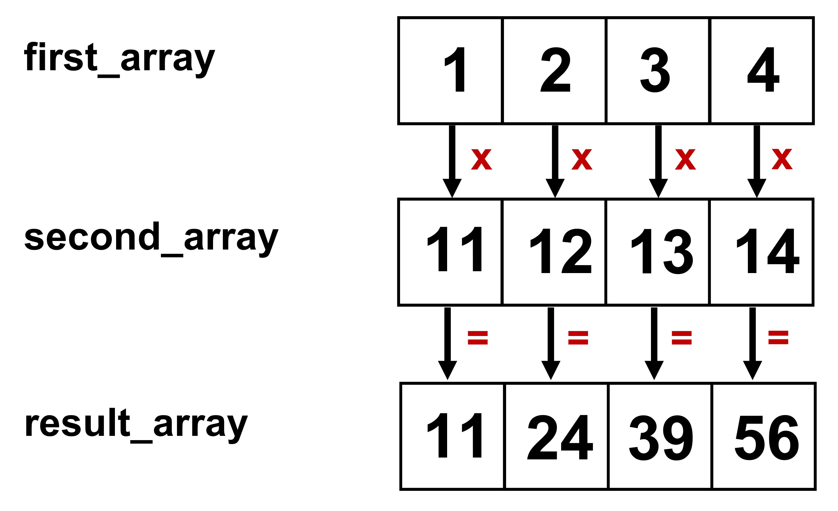
Fig. 7.1 Element-wise multiplication

7.1.6.1.2. Comparison

Comparison between an array and a number or another array happens element-wise as well. The result will be another array that will contain boolean values indicating whether the condition holds for each element or not. For example:

first_array < second_array

array([ True,  True,  True,  True])

In this case, first_array contains values [1,2,3,4] and second_array contains values [11,12,13,14]. Since 1 < 11, 2 < 12, 3 < 13 and 4 < 14, the resulting array will contain 4 True values.

What happens if the two arrays do not have the same shape?

third_array = np.arange(3,10)
first_array < third_array

---------------------------------------------------------------------------
ValueError                                Traceback (most recent call last)
Cell In[41], line 2
      1 third_array = np.arange(3,10)
----> 2 first_array < third_array

ValueError: operands could not be broadcast together with shapes (4,) (7,) 

In this case, a ValueError is raised indicating that the two operands of the < operator must have the same shape.

7.1.6.2. Axis calculations

Sometimes, we might need to perform data analysis with arrays that might have more than one dimension. Numpy offers many aggregate methods that include min(), max(), mean(), std(), etc. to find in an array-wise manner the minimum, maximum, mean and standard deviation of the array values, respectively. However, it is also possible that we might need to do these operations row- or column-wise. For this we can use the notion of axis. Axis determines on which direction we are making the calculations. In the case of 2D arrays, it takes value either 0 or 1. If axis=0, then the operation will be performed column-wise, meaning that for each column, the corresponding row values will be aggregated (go vertically). If on the other hand, axis=1, then the operation will be row-wise, this means that for each row, the corresponding column values will be aggregated (go horizontally). Fig. 7.2 illustrates the idea when we want to find the minimum vale:

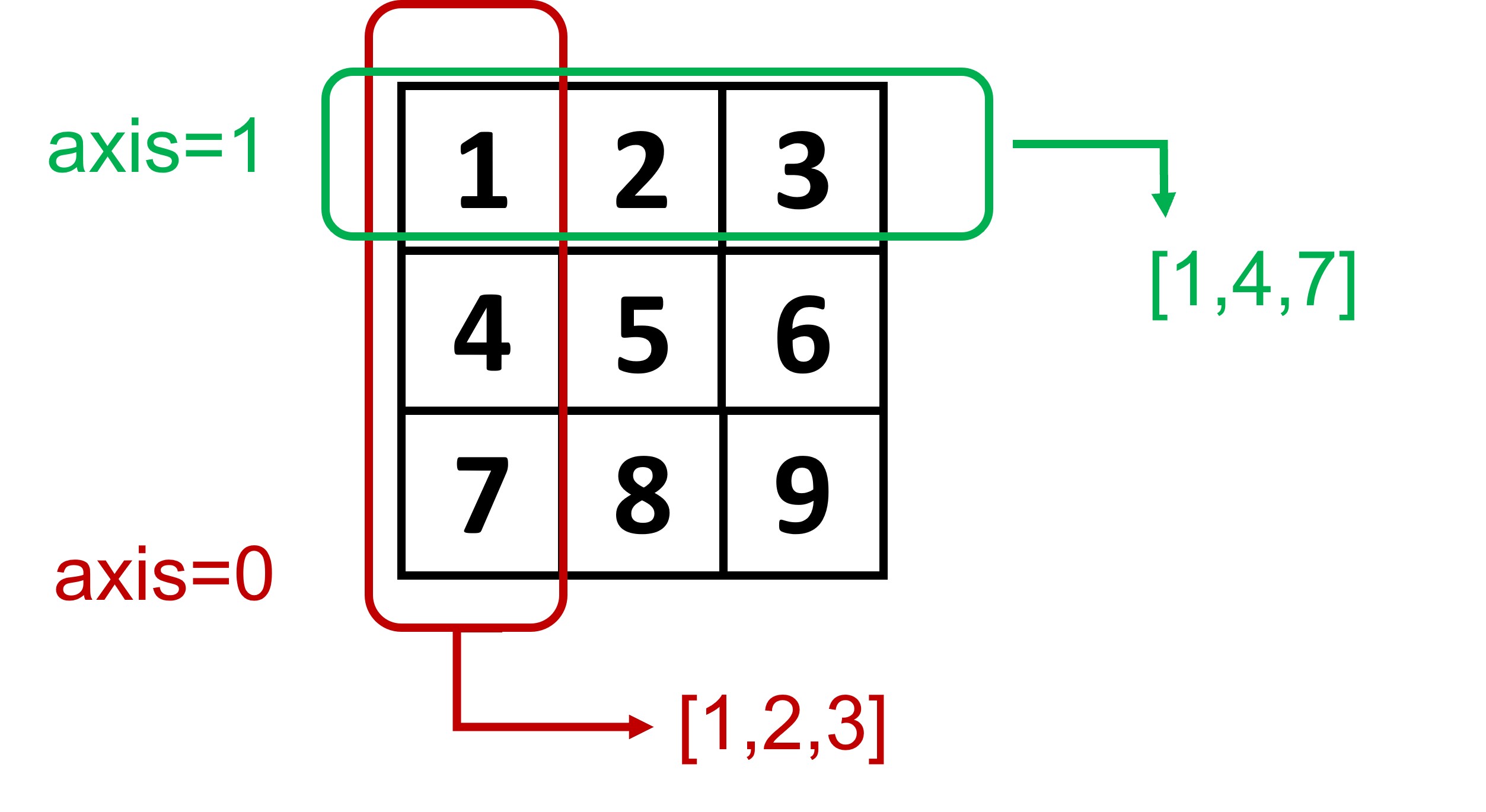
Fig. 7.2 Axis operations

In code, this would look like:

array = np.arange(1,10).reshape(3,3)
print('Minimum per row: ', array.min(axis = 1))
print('Minimum per column: ', array.min(axis = 0))

Minimum per row:  [1 4 7]
Minimum per column:  [1 2 3]

7.1.6.3. Other functions

Most of the arithmetic operations above can be performed using already built-in function from the numpy library. You can find a list of the functions in the Official Documentation of NumPy.

7.1.7. Slicing

Both indexing and slicing for one-dimensional arrays work the same as for lists in Chapter 5. Here we will focus on how we can index and slice two-dimensional arrays. The syntax is very similar to the one-dimensional case. However, now we need to specify two values or two ranges of values:

two_dim_array[row, col]

or

two_dim_array[row_range, col_range]

Let us look at some examples. Suppose we have the 3x3 array from the previous example:

array_2d = np.arange(1,10).reshape(3,3)
array_2d

array([[1, 2, 3],
       [4, 5, 6],
       [7, 8, 9]])

Reminder

Python arrays are 0-index-based as well.

In order to select the item in the second row and second column (the number 5 in this case), we need to write:

array_2d[1, 1]

5

The first number is used to select the row and the second one the column. In order to select the last two elements of the first two rows we would write:

array_2d[:2, 1:]

array([[2, 3],
       [5, 6]])

The first range selector :2 in English means: select all rows starting from the first up until but not including row 2 (0-based indexing). The second, column range selector 1: means, select all the column values from index 1 up until the end. Fig. 7.3 illustrates the idea:

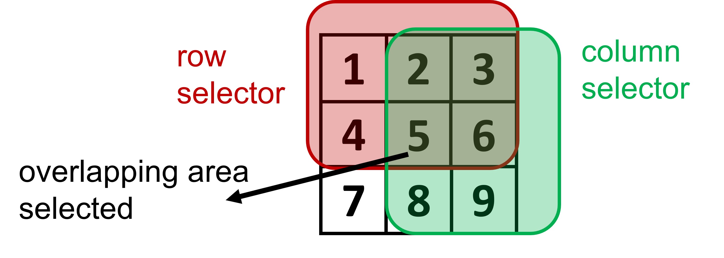
Fig. 7.3 Indexing in 2D arrays

If we want to select an entire row, we can specify only the index of the row we want to select:

array_2d[1]

array([4, 5, 6])

While if we want to select a specific column, we have to select all rows first and then provide the column index:

array_2d[:, 1]

array([2, 5, 8])

We can also select non-consecutive elements. For example:

array_2d[[0,2], :]

array([[1, 2, 3],
       [7, 8, 9]])

As you can see, the above code will first select the first and last rows and for each of this rows, will select all columns.

Important

However, when we pass two lists for selecting rows and columns, something interesting happens. As you can see from the code snippet below, only elements 1 and 9 are selected in this case. The reason why this happens is that element-wise slicing will happen. So for row 0 it is going to select element 0 and for row 2 it is going to select element at position 2, which is 9. You can think of the slicing part as: 0,0, 2,2, in terms of element selection.

array_2d[[0,2], [0,2]]

array([1, 9])

In the exercises we will build on this idea and show a way how to select more than two elements.